The (force-free) LBM equation is
f i ( x + c i , t + δ t ) − f i ( x , t ) = Ω i ( x , t ) . f_{i}(\boldsymbol{x} + \boldsymbol{c}_{i}, t+\delta_t) - f_{i}(\boldsymbol{x}, t) = \Omega_{i}(\boldsymbol{x}, t).
f i ( x + c i , t + δ t ) − f i ( x , t ) = Ω i ( x , t ) .
In LBGK model, Ω i ( x , t ) = − 1 τ [ f i ( x , t ) − f i ( e q ) ] \Omega_{i}(\boldsymbol{x}, t) = -\frac{1}{\tau} \left[ f_{i}(\boldsymbol{x}, t) - f_{i}^{(eq)} \right] Ω i ( x , t ) = − τ 1 [ f i ( x , t ) − f i ( e q ) ]
The f i ( e q ) f_{i}^{(eq)} f i ( e q )
f i ( e q ) = w i ρ [ 1 + c i ⋅ u c s 2 + ( c i ⋅ u ) 2 2 c s 4 − ∣ u ∣ 2 2 c s 2 ] . f_{i}^{(eq)} = w_{i} \rho \left[
1 + \frac{\boldsymbol{c}_{i} \cdot \boldsymbol{u}}{c_s^2}
+ \frac{(\boldsymbol{c}_{i} \cdot \boldsymbol{u})^2}{2 c_s^4}
- \frac{|\boldsymbol{u}|^2}{2 c_s^2}
\right].
f i ( e q ) = w i ρ [ 1 + c s 2 c i ⋅ u + 2 c s 4 ( c i ⋅ u ) 2 − 2 c s 2 ∣ u ∣ 2 ] .
w i w_i w i c i \boldsymbol{c}_{i} c i c s c_s c s ρ , u \rho, \boldsymbol{u} ρ , u
For simplicity, we define f i ∗ = f i − Ω i f^{*}_{i} = f_{i} - \Omega_{i} f i ∗ = f i − Ω i
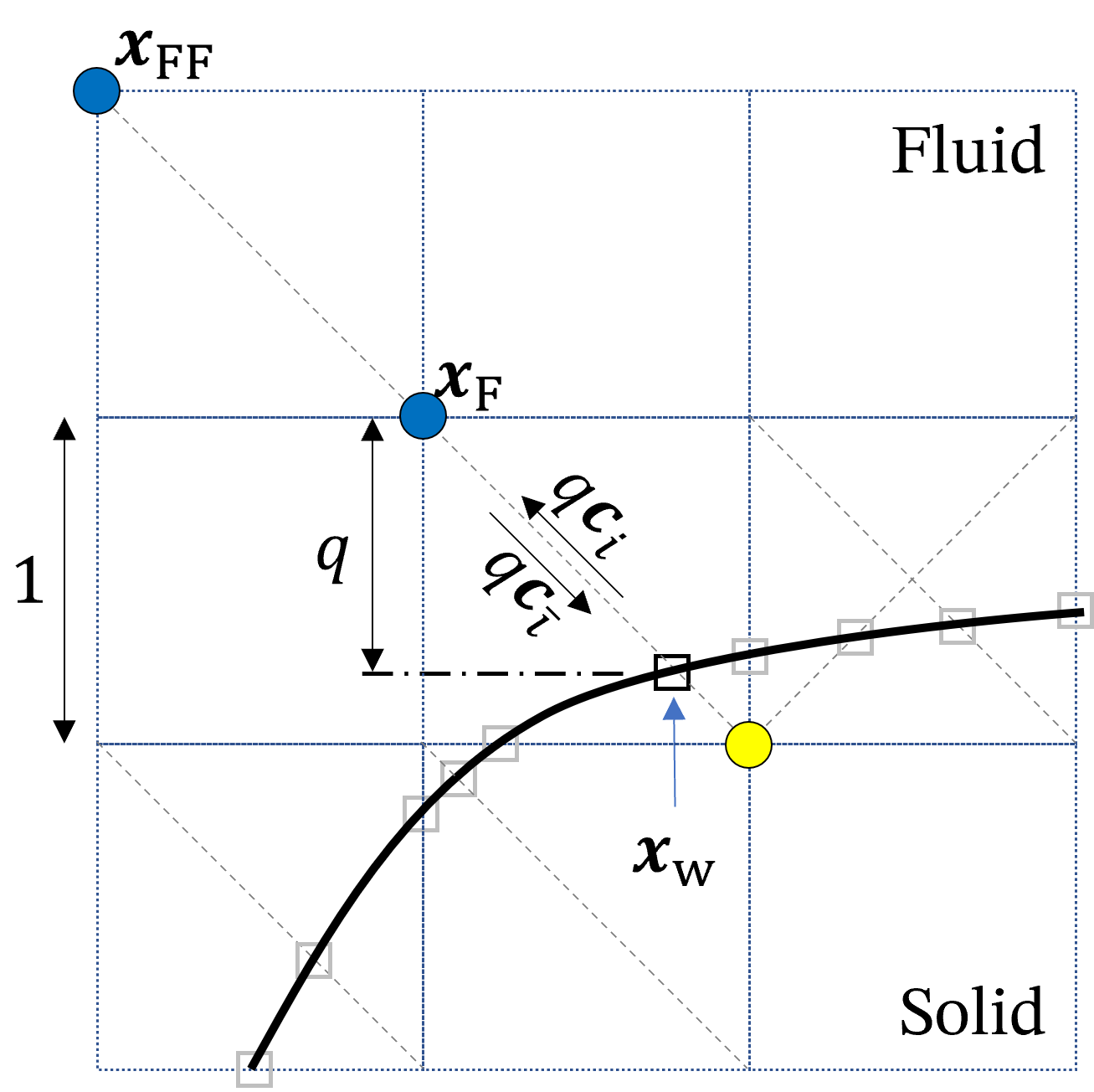
The purpose of boundary algorithms is to reconstruct missing f i ˉ ( x F , t + δ t ) f_{\bar{i}}(\boldsymbol{x}_{F}, t+\delta_t) f i ˉ ( x F , t + δ t )
Interpolated bounce-back method (IBB) ia a general ideas to implement the boundary condition. We will introduce it at below.
NOTE: ① In the left figure, x w = x F + q c i ˉ \boldsymbol{x}_{w} = \boldsymbol{x}_{F} + q \boldsymbol{c}_{\bar{i}} x w = x F + q c i ˉ c i ˉ = − c i \boldsymbol{c}_{\bar{i}} = -\boldsymbol{c}_{i} c i ˉ = − c i x ⃗ b \vec{x}_b x b q = ∣ x ⃗ w − x ⃗ F ∣ / ∣ x ⃗ b − x ⃗ F ∣ q = |\vec{x}_w - \vec{x}_F| / |\vec{x}_b - \vec{x}_F| q = ∣ x w − x F ∣ / ∣ x b − x F ∣
It treats the unknown f i ( x F , t + δ t ) f_{i}(\boldsymbol{x}_{F}, t+\delta_t) f i ( x F , t + δ t )
f i ( x F , t + δ t ) = a 1 f i ˉ ∗ ( x F F , t ) + a 2 f i ˉ ∗ ( x F , t ) + a 3 f i ∗ ( x F , t ) + K f_{i}(\boldsymbol{x}_{F}, t+\delta_t) =
a_1 f_{\bar{i}}^{*}(\boldsymbol{x}_{FF}, t) +
a_2 f_{\bar{i}}^{*}(\boldsymbol{x}_{F}, t) + a_3 f_{i}^{*}(\boldsymbol{x}_{F}, t) + K
f i ( x F , t + δ t ) = a 1 f i ˉ ∗ ( x F F , t ) + a 2 f i ˉ ∗ ( x F , t ) + a 3 f i ∗ ( x F , t ) + K
where K K K
|👉 How to find the coefficients a i a_i a i
It determinates the boundary scheme based on the value of q q q
When q ≥ 1 2 q \ge \frac{1}{2} q ≥ 2 1
f i ( x + , t + δ t ) = f i ˉ ∗ ( x F , t ) , f i ( x F F , t + δ t ) = f i ∗ ( x F , t ) . f_{i}(\boldsymbol{x}_{+}, t+\delta_t) = f_{\bar{i}}^{*} (\boldsymbol{x}_{F}, t)
,\quad
f_{i}(\boldsymbol{x}_{FF}, t+\delta_t) = f_{i}^{*} (\boldsymbol{x}_{F}, t).
f i ( x + , t + δ t ) = f i ˉ ∗ ( x F , t ) , f i ( x F F , t + δ t ) = f i ∗ ( x F , t ) .
Then we can do linear interpolation to calculate f i ( x F , t + δ t ) f_{i}(\boldsymbol{x}_{F}, t+\delta_t) f i ( x F , t + δ t )
f i ( x F , t + δ t ) = f i ( x + , t + δ t ) + 2 q − 1 2 q [ f i ( x F F , t + δ t ) − f i ( x + , t + δ t ) ] = 1 2 q f i ˉ ∗ ( x F , t ) + ( 1 − 1 2 q ) f i ∗ ( x F , t ) \begin{aligned}
f_{i}(\boldsymbol{x}_{F}, t+\delta_t) =& f_{i}(\boldsymbol{x}_{+}, t+\delta_t) + \\
&\frac{2q - 1}{2q} [f_{i}(\boldsymbol{x}_{FF}, t+\delta_t)- f_{i}(\boldsymbol{x}_{+}, t+\delta_t)] \\
=& \frac{1}{2q} f_{\bar{i}}^{*} (\boldsymbol{x}_{F}, t) + (1-\frac{1}{2q}) f_{i}^{*} (\boldsymbol{x}_{F}, t)
\end{aligned}
f i ( x F , t + δ t ) = = f i ( x + , t + δ t ) + 2 q 2 q − 1 [ f i ( x F F , t + δ t ) − f i ( x + , t + δ t ) ] 2 q 1 f i ˉ ∗ ( x F , t ) + ( 1 − 2 q 1 ) f i ∗ ( x F , t )
When q < 1 2 q < \frac{1}{2} q < 2 1
f i ( x F , t + δ t ) = f i ˉ ∗ ( x + , t ) = f i ˉ ∗ ( x F , t ) + ( 1 − 2 q ) [ f i ˉ ∗ ( x F F , t ) − f i ˉ ∗ ( x F , t ) ] = 2 q f i ˉ ∗ ( x F , t ) + ( 1 − 2 q ) f i ˉ ∗ ( x F F , t ) \begin{aligned}
f_{i}(\boldsymbol{x}_{F}, t+\delta_t) =& f_{\bar{i}}^{*}(\boldsymbol{x}_{+}, t)\\
=& f_{\bar{i}}^{*}(\boldsymbol{x}_{F}, t) \\
& + (1-2q) [f_{\bar{i}}^{*}(\boldsymbol{x}_{FF}, t) - f_{\bar{i}}^{*}(\boldsymbol{x}_{F}, t)]\\
=& 2q f_{\bar{i}}^{*}(\boldsymbol{x}_{F}, t) + (1-2q) f_{\bar{i}}^{*}(\boldsymbol{x}_{FF}, t)
\end{aligned}
f i ( x F , t + δ t ) = = = f i ˉ ∗ ( x + , t ) f i ˉ ∗ ( x F , t ) + ( 1 − 2 q ) [ f i ˉ ∗ ( x F F , t ) − f i ˉ ∗ ( x F , t ) ] 2 q f i ˉ ∗ ( x F , t ) + ( 1 − 2 q ) f i ˉ ∗ ( x F F , t )
We can notice that: the general scheme usually employs the data of x F F \boldsymbol{x}_{FF} x F F
To design local linkwise boundary condition, one must discard the nonlocal contribution f ∗ ( x F F , t ) f^{*}(\boldsymbol{x}_{FF}, t) f ∗ ( x F F , t )
Because the existence of f ∗ ( x F F , t ) f^{*}(\boldsymbol{x}_{FF}, t) f ∗ ( x F F , t )
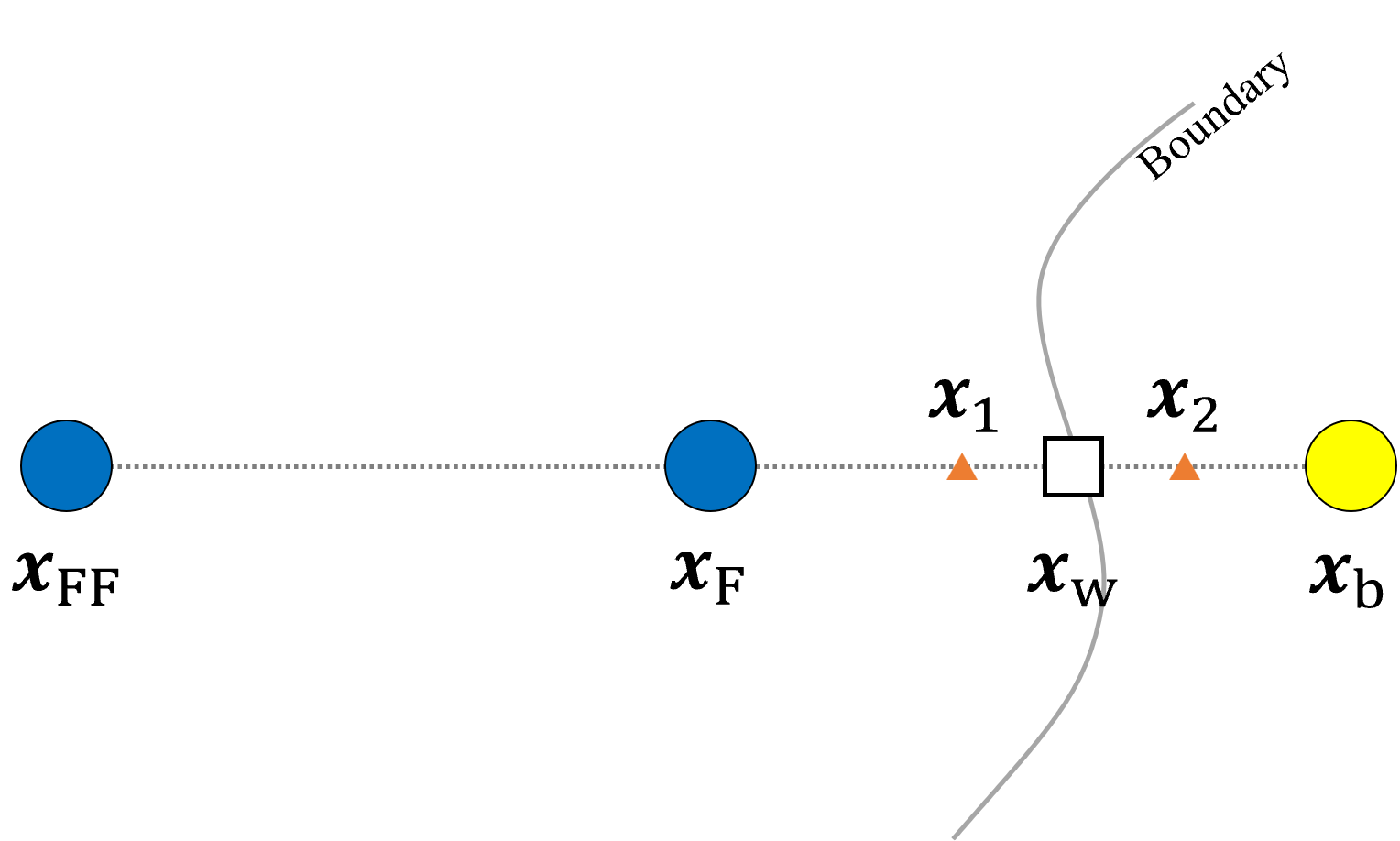
The boundary node x ⃗ w \vec{x}_w x w x ⃗ 1 \vec{x}_1 x 1 x ⃗ 2 \vec{x}_2 x 2 (J. Fluid Mech. , 271 (1994), pp. 285–309) .
The first one is based on the following first-order in time approximation:
f i ˉ ∗ ( x F F , t ) = f i ˉ ( x F , t + δ t ) ⏟ LBM streaming step ≈ f i ˉ ( x F , t ) ⏟ Approximation \underbrace{f_{\bar{i}}^{*}(\boldsymbol{x}_{FF}, t) = f_{\bar{i}}(\boldsymbol{x}_{F}, t+\delta_t) }_{\text{LBM streaming step}}
\approx
\underbrace{f_{\bar{i}}(\boldsymbol{x}_{F}, t)}_{\text{Approximation}}
LBM streaming step f i ˉ ∗ ( x F F , t ) = f i ˉ ( x F , t + δ t ) ≈ Approximation f i ˉ ( x F , t )
Zhao et al.[3] point out that: their scheme can obtain second-order accuracy under the diffusive scaling (δ t = O ( δ x 2 ) \delta_t = O(\delta_x^2) δ t = O ( δ x 2 )
Here:
x ⃗ w = x ⃗ F + q c ⃗ i ˉ \vec{x}_w = \vec{x}_{F} + q \vec{c}_{\bar{i}} x w = x F + q c i ˉ x ⃗ 1 = x ⃗ F + l c ⃗ i ˉ \vec{x}_1 = \vec{x}_{F} + l \vec{c}_{\bar{i}} x 1 = x F + l c i ˉ x ⃗ 2 = 2 x ⃗ w − x ⃗ 1 \vec{x}_2 = 2 \vec{x}_{w} - \vec{x}_1 x 2 = 2 x w − x 1
Stability condition: l ∈ [ max { 0 , 2 q − 1 } , 2 q ] l \in [\max\{0, 2q-1\}, 2q] l ∈ [ max { 0 , 2 q − 1 } , 2 q ]
With x ⃗ 1 \vec{x}_1 x 1 x ⃗ F F \vec{x}_{FF} x F F x ⃗ F \vec{x}_{F} x F
f i ( x ⃗ F , t + δ t ) = l 1 + l f i ( x ⃗ F F , t + δ t ) + 1 1 + l f i ( x ⃗ 1 , t + δ t ) = l 1 + l f i ∗ ( x ⃗ F , t ) ⏟ LBM Streaming + 1 1 + l f i ( x ⃗ 1 , t + δ t ) \begin{aligned}
f_i (\vec{x}_{F}, t + \delta_t) =& \frac{l}{1+l} f_i (\vec{x}_{FF}, t + \delta_t) + \frac{1}{1+l} f_i (\vec{x}_{1}, t + \delta_t) \\
=& \underbrace{\frac{l}{1+l} f_i^{*} (\vec{x}_{F}, t)}_{\text{LBM Streaming}} + \frac{1}{1+l} f_i (\vec{x}_{1}, t + \delta_t)
\end{aligned}
f i ( x F , t + δ t ) = = 1 + l l f i ( x F F , t + δ t ) + 1 + l 1 f i ( x 1 , t + δ t ) LBM Streaming 1 + l l f i ∗ ( x F , t ) + 1 + l 1 f i ( x 1 , t + δ t )
For the unknown distribution function f i ( x ⃗ 1 , t + δ t ) f_i (\vec{x}_{1}, t + \delta_t) f i ( x 1 , t + δ t ) (J. Fluid Mech. , 271 (1994), pp. 285–309) .
f i ( x ⃗ 1 , t + δ t ) = f i ˉ ( x ⃗ 2 , t + δ t ) + 2 w i ρ 0 c i ⋅ u ( x ⃗ b , t ) c s 2 f_i (\vec{x}_{1}, t + \delta_t) =
f_{\bar{i}} (\vec{x}_{2}, t + \delta_t) + 2 w_i \rho_0 \frac{\boldsymbol{c}_i \cdot \boldsymbol{u}(\vec{x}_b, t)}{c_s^2}
f i ( x 1 , t + δ t ) = f i ˉ ( x 2 , t + δ t ) + 2 w i ρ 0 c s 2 c i ⋅ u ( x b , t )
Here the wall velocity u ( x ⃗ b , t ) \boldsymbol{u}(\vec{x}_b, t) u ( x b , t )
Next, we interpolate f i ˉ ( x ⃗ 2 , t + δ t ) f_{\bar{i}} (\vec{x}_{2}, t + \delta_t) f i ˉ ( x 2 , t + δ t ) x ⃗ F \vec{x}_F x F x ⃗ b \vec{x}_b x b
f i ˉ ( x ⃗ 2 , t + δ t ) = ( 1 + l − 2 q ) f i ˉ ( x ⃗ F , t + δ t ) + ( 2 q − l ) f i ˉ ( x ⃗ b , t + δ t ) f_{\bar{i}} (\vec{x}_{2}, t + \delta_t) =
(1+l-2q) f_{\bar{i}} (\vec{x}_{F}, t + \delta_t) +
(2q-l) f_{\bar{i}} (\vec{x}_{b}, t + \delta_t)
f i ˉ ( x 2 , t + δ t ) = ( 1 + l − 2 q ) f i ˉ ( x F , t + δ t ) + ( 2 q − l ) f i ˉ ( x b , t + δ t )
Consider the streaming step from x ⃗ F \vec{x}_F x F x ⃗ b \vec{x}_b x b f i ˉ ∗ ( x ⃗ F , t ) = f i ˉ ( x ⃗ b , t + δ t ) f_{\bar{i}}^{*} (\vec{x}_{F}, t) = f_{\bar{i}} (\vec{x}_{b}, t + \delta_t) f i ˉ ∗ ( x F , t ) = f i ˉ ( x b , t + δ t )
Finally, with the approximation
f i ˉ ∗ ( x F F , t ) = f i ˉ ( x F , t + δ t ) ⏟ LBM streaming step ≈ f i ˉ ( x F , t ) ⏟ Approximation , \underbrace{f_{\bar{i}}^{*}(\boldsymbol{x}_{FF}, t) = f_{\bar{i}}(\boldsymbol{x}_{F}, t+\delta_t) }_{\text{LBM streaming step}}
\approx
\underbrace{f_{\bar{i}}(\boldsymbol{x}_{F}, t)}_{\text{Approximation}},
LBM streaming step f i ˉ ∗ ( x F F , t ) = f i ˉ ( x F , t + δ t ) ≈ Approximation f i ˉ ( x F , t ) ,
we can obtain the local boundary scheme:
f i ( x ⃗ F , t + δ t ) = 1 + l − 2 q 1 + l f i ˉ ( x ⃗ F , t ) ⏟ before collision + l 1 + l f i ∗ ( x F , t ) + 2 q − l 1 + l f i ˉ ∗ ( x F , t ) ⏟ post collision terms + 2 w i ρ 0 ( 1 + l ) c s 2 c i ⋅ u ( x ⃗ b , t ) ⏟ Ladd’s bounce-back f_i (\vec{x}_{F}, t + \delta_t) =
\underbrace{
\frac{1+l-2q}{1+l} f_{\bar{i}} (\vec{x}_F, t)
}_{\text{before collision}} +
\underbrace{
\frac{l}{1+l} f_{i}^{*}(\boldsymbol{x}_{F}, t) +
\frac{2q-l}{1+l} f_{\bar{i}}^{*}(\boldsymbol{x}_{F}, t)
}_{\text{post collision terms}} +
\underbrace{\frac{2 w_i \rho_0}{(1+l)c_s^2} \boldsymbol{c}_i \cdot \boldsymbol{u}(\vec{x}_b, t)}_{\text{Ladd's bounce-back}}
f i ( x F , t + δ t ) = before collision 1 + l 1 + l − 2 q f i ˉ ( x F , t ) + post collision terms 1 + l l f i ∗ ( x F , t ) + 1 + l 2 q − l f i ˉ ∗ ( x F , t ) + Ladd’s bounce-back ( 1 + l ) c s 2 2 w i ρ 0 c i ⋅ u ( x b , t )
[NOTE] x F F \boldsymbol{x}_{FF} x F F l = q l = q l = q (Comput. Math. Appl. , 70 (2015), pp. 507–547)
f i ( x ⃗ F , t + δ t ) = 1 − q 1 + q f i ˉ ( x ⃗ F , t ) + q 1 + q [ f i ∗ ( x F , t ) + f i ˉ ∗ ( x F , t ) ] + 2 w i ρ 0 ( 1 + q ) c s 2 c i ⋅ u ( x ⃗ b , t ) f_i (\vec{x}_{F}, t + \delta_t) =
\frac{1-q}{1+q} f_{\bar{i}} (\vec{x}_F, t) +
\frac{q}{1+q} [f_{i}^{*}(\boldsymbol{x}_{F}, t) +
f_{\bar{i}}^{*}(\boldsymbol{x}_{F}, t)] +
\frac{2 w_i \rho_0}{(1+q)c_s^2}
\boldsymbol{c}_i \cdot \boldsymbol{u}(\vec{x}_b, t)
f i ( x F , t + δ t ) = 1 + q 1 − q f i ˉ ( x F , t ) + 1 + q q [ f i ∗ ( x F , t ) + f i ˉ ∗ ( x F , t ) ] + ( 1 + q ) c s 2 2 w i ρ 0 c i ⋅ u ( x b , t )
If we still use f i ˉ ∗ ( x ⃗ F F , t ) f_{\bar{i}}^{*} (\vec{x}_{FF}, t) f i ˉ ∗ ( x F F , t ) f i ˉ ( x ⃗ F , t ) f_{\bar{i}} (\vec{x}_{F}, t) f i ˉ ( x F , t ) (AIAA Paper , 2003-0953, 2003.) .
Tao et al.[4] have proposed a scheme to reconstruct the equilibrium and non-equilibrium state of the fluid node near the wall.
For the boundary node x ⃗ F \vec{x}_F x F
f i ( x ⃗ F , t + δ t ) = 1 1 + q f i ( x ⃗ w , t + δ t ) + q 1 + q f i ( x ⃗ F F , t + δ t ) . f_{i}(\vec{x}_F, t + \delta_t) = \frac{1}{1+q} f_{i}(\vec{x}_w, t + \delta_t) +
\frac{q}{1+q} f_{i}(\vec{x}_{FF}, t + \delta_t).
f i ( x F , t + δ t ) = 1 + q 1 f i ( x w , t + δ t ) + 1 + q q f i ( x F F , t + δ t ) .
Then we begin to discuss the reconstruction process.
First, consider the streaming step from x ⃗ F \vec{x}_F x F x ⃗ F F \vec{x}_{FF} x F F
f i ∗ ( x ⃗ F , t ) = f i ( x ⃗ F F , t + δ t ) f_{i}^{*}(\vec{x}_{F}, t) = f_{i}(\vec{x}_{FF}, t + \delta_t)
f i ∗ ( x F , t ) = f i ( x F F , t + δ t )
Second, the term f i ( x ⃗ w , t + δ t ) f_{i}(\vec{x}_w, t + \delta_t) f i ( x w , t + δ t ) f i ( e q ) f_{i}^{(eq)} f i ( e q ) f i ( n e q ) f_{i}^{(neq)} f i ( n e q )
f i ( x ⃗ w , t + δ t ) = f i ( e q ) ( x ⃗ w , t + δ t ) + f i ( n e q ) ( x ⃗ w , t + δ t ) = f i ( e q ) ( x ⃗ w , t + δ t ) + f i ( n e q ) ( x ⃗ F , t + δ t ) = f i ( e q ) ( x ⃗ w , t + δ t ) + f i ˉ ( n e q ) ( x ⃗ F , t ) \begin{aligned}
f_{i}(\vec{x}_w, t + \delta_t) &= f_{i}^{(eq)}(\vec{x}_w, t + \delta_t) + f_{i}^{(neq)}(\vec{x}_w, t + \delta_t) \\
&= f_{i}^{(eq)}(\vec{x}_w, t + \delta_t) + f_{i}^{(neq)}(\vec{x}_F, t + \delta_t) \\
&= f_{i}^{(eq)}(\vec{x}_w, t + \delta_t) + f_{\bar{i}}^{(neq)}(\vec{x}_F, t)
\end{aligned}
f i ( x w , t + δ t ) = f i ( e q ) ( x w , t + δ t ) + f i ( n e q ) ( x w , t + δ t ) = f i ( e q ) ( x w , t + δ t ) + f i ( n e q ) ( x F , t + δ t ) = f i ( e q ) ( x w , t + δ t ) + f i ˉ ( n e q ) ( x F , t )
Consider the substitution from f i ( n e q ) ( x ⃗ F , t + δ t ) f_{i}^{(neq)}(\vec{x}_F, t + \delta_t) f i ( n e q ) ( x F , t + δ t ) f i ˉ ( n e q ) ( x ⃗ F , t ) f_{\bar{i}}^{(neq)}(\vec{x}_F, t) f i ˉ ( n e q ) ( x F , t ) as mentioned in Tao et al.[4].
The f i ( e q ) ( x ⃗ w , t + δ t ) f_{i}^{(eq)}(\vec{x}_w, t + \delta_t) f i ( e q ) ( x w , t + δ t )
f i ( e q ) ( x ⃗ w , t + δ t ) = f i ( e q ) ( u ⃗ ( x ⃗ w , t + δ t ) , ρ ( x ⃗ w , t + δ t ) ) ≈ f i ( e q ) ( u ⃗ ( x ⃗ w , t + δ t ) , ρ ( x ⃗ F , t + δ t ) ) ≈ f i ( e q ) ( u ⃗ ( x ⃗ w , t + δ t ) , ρ ( x ⃗ F , t ) ) \begin{aligned}
f_{i}^{(eq)}(\vec{x}_w, t + \delta_t) &= f_{i}^{(eq)} \left( \vec{u}(\vec{x}_w, t + \delta_t), \rho(\vec{x}_w, t + \delta_t) \right) \\
&\approx f_{i}^{(eq)} \left( \vec{u}(\vec{x}_w, t + \delta_t), \rho(\vec{x}_F, t + \delta_t) \right) \\
&\approx f_{i}^{(eq)} \left( \vec{u}(\vec{x}_w, t + \delta_t), \rho(\vec{x}_F, t) \right) \\
\end{aligned}
f i ( e q ) ( x w , t + δ t ) = f i ( e q ) ( u ( x w , t + δ t ) , ρ ( x w , t + δ t ) ) ≈ f i ( e q ) ( u ( x w , t + δ t ) , ρ ( x F , t + δ t ) ) ≈ f i ( e q ) ( u ( x w , t + δ t ) , ρ ( x F , t ) )
Here we cite the original sentences from the paper [4]:
It has been demonstrated that for low speed flow, using ρ A ( t ) \rho_A (t) ρ A ( t ) ρ A ( t + δ t ) \rho_A (t+\delta_t) ρ A ( t + δ t ) ρ A ( t + δ t ) \rho_A (t+\delta_t) ρ A ( t + δ t ) ρ W ( t + δ t ) \rho_W (t+\delta_t) ρ W ( t + δ t )
== Reference ==
So the boundary scheme purposed by Tao et al. [4] is:
f i ( x ⃗ F , t + δ t ) = q 1 + q f i ∗ ( x ⃗ F , t ) + 1 1 + q { f i ( e q ) ( u ⃗ ( x ⃗ w , t + δ t ) , ρ ( x ⃗ F , t ) ) + f i ˉ ( n e q ) ( x ⃗ F , t ) } f_{i}(\vec{x}_F, t + \delta_t) =
\frac{q}{1+q} f_{i}^{*}(\vec{x}_{F}, t) +
\frac{1}{1+q} \left\{ f_{i}^{(eq)} \left( \vec{u}(\vec{x}_w, t + \delta_t), \rho(\vec{x}_F, t) \right) + f_{\bar{i}}^{(neq)}(\vec{x}_F, t) \right\}
f i ( x F , t + δ t ) = 1 + q q f i ∗ ( x F , t ) + 1 + q 1 { f i ( e q ) ( u ( x w , t + δ t ) , ρ ( x F , t ) ) + f i ˉ ( n e q ) ( x F , t ) }
[NOTE] f i ( x ⃗ F F , t + δ t ) f_{i}(\vec{x}_{FF}, t + \delta_t) f i ( x F F , t + δ t ) x ⃗ w \vec{x}_w x w f i ( e q ) f_{i}^{(eq)} f i ( e q ) f i ( n e q ) f_{i}^{(neq)} f i ( n e q ) f i ( e q ) f_{i}^{(eq)} f i ( e q ) f i ( n e q ) f_{i}^{(neq)} f i ( n e q )
Here, we introduce the enhanced single-node boundary condition purposed by Marson et al.[1].
f i ( x ⃗ F , t + δ t ) = a 1 f i ˉ ∗ ( x ⃗ F F ) + a 2 ( x ⃗ F + 2 f ( e q ) − ( x ⃗ w ) ) ⏟ 1 + a 3 f i ∗ ( x ⃗ F ) + a 4 f ~ i ( x ⃗ w , t + δ t ) ⏟ 2 + a 5 f ~ i ∗ ( x ⃗ w ) ⏟ 3 − K − f i ( n e q ) − ( x ⃗ F ) τ − ⏟ 4 \begin{aligned}
f_{i}(\vec{x}_F, t + \delta_t) =& \cancel{a_1 f_{\bar{i}}^{*}(\vec{x}_{FF})} +
a_2 \underbrace{(\vec{x}_{F} + 2 f^{(eq)-}(\vec{x}_{w}))}_{\text{1}} + a_3 f_{i}^{*}(\vec{x}_{F})\\
& + a_4 \underbrace{ \tilde{f}_{i}(\vec{x}_w, t + \delta_t) }_{\text{2}} + a_5 \underbrace{\tilde{f}_{i}^{*}(\vec{x}_w)}_{\text{3}} -
\underbrace{K^{-} \frac{f_{i}^{(neq)-}(\vec{x}_F)}{\tau^{-}}}_{\text{4}}
\end{aligned}
f i ( x F , t + δ t ) = a 1 f i ˉ ∗ ( x F F ) + a 2 1 ( x F + 2 f ( e q ) − ( x w ) ) + a 3 f i ∗ ( x F ) + a 4 2 f ~ i ( x w , t + δ t ) + a 5 3 f ~ i ∗ ( x w ) − 4 K − τ − f i ( n e q ) − ( x F )
Term ① : The haly-way bounce-back from Ladd (J. Fluid Mech. , 271 (1994), pp. 285–309) .f ( e q ) − ( x ⃗ w ) = w i ρ c ⃗ i ⋅ u ⃗ w / c s 2 f^{(eq)-}(\vec{x}_{w}) = w_i \rho \vec{c}_i \cdot \vec{u}_w / c_s^2 f ( e q ) − ( x w ) = w i ρ c i ⋅ u w / c s 2 Term ② : The term from [4].Term ③ : The new term designed by Marson et al.[1].Term ④ : The new (optional) term mentioned in the Sec. ⅣB of Marson et al.[1].
Marson et al.[1] use TRT collision model. So here we briefly introduce the two-relaxation-time (TRT) collision model.
{ f i + ( x ⃗ + c ⃗ i δ t , t + δ t ) − f i + ( x ⃗ , t ) = − 1 τ + ( f i + ( x ⃗ , t ) − f i ( e q ) + ( x ⃗ , t ) ) f i − ( x ⃗ + c ⃗ i δ t , t + δ t ) − f i − ( x ⃗ , t ) = − 1 τ − ( f i − ( x ⃗ , t ) − f i ( e q ) − ( x ⃗ , t ) ) \begin{cases}
f_{i}^{+} (\vec{x} + \vec{c}_i \delta_t, t + \delta_t) - f_{i}^{+} (\vec{x}, t)
= -\frac{1}{\tau^{+}} (f_{i}^{+} (\vec{x}, t) - f_{i}^{(eq)+} (\vec{x}, t)) \\
f_{i}^{-} (\vec{x} + \vec{c}_i \delta_t, t + \delta_t) - f_{i}^{-} (\vec{x}, t)
= -\frac{1}{\tau^{-}} (f_{i}^{-} (\vec{x}, t) - f_{i}^{(eq)-} (\vec{x}, t)) \\
\end{cases}
{ f i + ( x + c i δ t , t + δ t ) − f i + ( x , t ) = − τ + 1 ( f i + ( x , t ) − f i ( e q ) + ( x , t ) ) f i − ( x + c i δ t , t + δ t ) − f i − ( x , t ) = − τ − 1 ( f i − ( x , t ) − f i ( e q ) − ( x , t ) )
where
f i + = 1 2 ( f i + f − i ) , f i − = 1 2 ( f i − f − i ) , f i ( e q ) + = 1 2 ( f i ( e q ) + f − i ( e q ) ) = w i ρ ( 1 + ( c ⃗ i ⋅ u ⃗ ) 2 2 c s 4 − ∣ u ⃗ ∣ 2 2 c s 2 ) , f i ( e q ) − = 1 2 ( f i ( e q ) − f − i ( e q ) ) = w i ρ c ⃗ i ⋅ u ⃗ c s 2 , \begin{aligned}
f_{i}^{+} = \frac{1}{2} (f_i + f_{-i}) ,\quad
f_{i}^{-} = \frac{1}{2} (f_i - f_{-i}) ,\\
f_{i}^{(eq)+} = \frac{1}{2} (f_i^{(eq)} + f_{-i}^{(eq)})
= w_i \rho (1 + \frac{(\vec{c}_i \cdot \vec{u})^2}{2 c_s^4} - \frac{|\vec{u}|^2}{2 c_s^2})
,\\
f_{i}^{(eq)-} = \frac{1}{2} (f_i^{(eq)} - f_{-i}^{(eq)})
= w_i \rho \frac{\vec{c}_i \cdot \vec{u}}{c_s^2}
,\\
\end{aligned}
f i + = 2 1 ( f i + f − i ) , f i − = 2 1 ( f i − f − i ) , f i ( e q ) + = 2 1 ( f i ( e q ) + f − i ( e q ) ) = w i ρ ( 1 + 2 c s 4 ( c i ⋅ u ) 2 − 2 c s 2 ∣ u ∣ 2 ) , f i ( e q ) − = 2 1 ( f i ( e q ) − f − i ( e q ) ) = w i ρ c s 2 c i ⋅ u ,
and the TRT magic number is: Λ = ( τ + − 1 2 ) ( τ − − 1 2 ) \Lambda = (\tau^{+} - \frac{1}{2}) (\tau^{-} - \frac{1}{2}) Λ = ( τ + − 2 1 ) ( τ − − 2 1 )
Marson et al.[1] design the wall populations f ~ i ∗ ( x ⃗ w ) \tilde{f}_{i}^{*}(\vec{x}_w) f ~ i ∗ ( x w ) f ~ i ( x ⃗ w , t + δ t ) \tilde{f}_{i}(\vec{x}_w, t+\delta_t) f ~ i ( x w , t + δ t ) Ω \Omega Ω
f ~ i ∗ ( x ⃗ w , t ) = def f ~ i ( e q ) ( x ⃗ w , t ) + ( 1 − Ω ) f ~ i ( n e q ) ( x ⃗ w , t ) f ~ i ( x ⃗ w , t + δ t ) = def f ~ i ( e q ) ( x ⃗ w , t + δ t ) + f ~ i ( n e q ) ( x ⃗ w , t + δ t ) \begin{aligned}
\tilde{f}_{i}^{*}(\vec{x}_w, t) \overset{\text{def}}{=}& \tilde{f}_{i}^{(eq)}(\vec{x}_w, t) + (1 - \Omega) \tilde{f}_{i}^{(neq)}(\vec{x}_w, t) \\
\tilde{f}_{i}(\vec{x}_w, t+\delta_t) \overset{\text{def}}{=}& \tilde{f}_{i}^{(eq)}(\vec{x}_w, t+\delta_t) + \tilde{f}_{i}^{(neq)}(\vec{x}_w, t+\delta_t)
\end{aligned}
f ~ i ∗ ( x w , t ) = def f ~ i ( x w , t + δ t ) = def f ~ i ( e q ) ( x w , t ) + ( 1 − Ω ) f ~ i ( n e q ) ( x w , t ) f ~ i ( e q ) ( x w , t + δ t ) + f ~ i ( n e q ) ( x w , t + δ t )
Consider f ~ i ( x ⃗ w , t + δ t ) \tilde{f}_{i}(\vec{x}_w, t+\delta_t) f ~ i ( x w , t + δ t )
f ~ i ( e q ) ( x ⃗ w , t + δ t ) ≈ f i ( e q ) + ( ρ ( x ⃗ F , t ) , u ⃗ ( x ⃗ { w , F } , t + δ t ) ) + f i ( e q ) − ( ρ ( x ⃗ F , t ) , u ⃗ ( x ⃗ w , t + δ t ) ) \tilde{f}_{i}^{(eq)} (\vec{x}_w, t+\delta_t) \approx
f_{i}^{(eq)+} (\rho(\vec{x}_F, t), \vec{u}(\vec{x}_{\{w, F\}}, t+\delta_t)) +
f_{i}^{(eq)-} (\rho(\vec{x}_F, t), \vec{u}(\vec{x}_{w}, t+\delta_t))
f ~ i ( e q ) ( x w , t + δ t ) ≈ f i ( e q ) + ( ρ ( x F , t ) , u ( x { w , F } , t + δ t ) ) + f i ( e q ) − ( ρ ( x F , t ) , u ( x w , t + δ t ) )
Here, x ⃗ { w , F } \vec{x}_{\{w, F\}} x { w , F } x ⃗ w \vec{x}_{w} x w x ⃗ F \vec{x}_F x F
The non-equilibrium part is approximated by an nonequilibrium bounce-back. This is a first-order approximation of the nonequilibrium bounce-back method of Zou and He, and it leads to the following second-order accurate approximation:
f ~ i ( n e q ) ( x ⃗ w , t + δ t ) = f ~ i ( n e q ) ( x ⃗ F , t ) \tilde{f}_{i}^{(neq)}(\vec{x}_w, t+\delta_t) = \tilde{f}_{i}^{(neq)}(\vec{x}_F, t)
f ~ i ( n e q ) ( x w , t + δ t ) = f ~ i ( n e q ) ( x F , t )
For the f ~ i ∗ ( x ⃗ w , t ) \tilde{f}_{i}^{*}(\vec{x}_w, t) f ~ i ∗ ( x w , t )
f ~ i ( e q ) ( x ⃗ w , t ) ≈ f i ( e q ) + ( ρ ( x ⃗ F , t ) , u ⃗ ( x ⃗ { w , F } , t ) ) + f i ( e q ) − ( ρ ( x ⃗ F , t ) , u ⃗ ( x ⃗ w , t ) ) \tilde{f}_{i}^{(eq)} (\vec{x}_w, t) \approx
f_{i}^{(eq)+} (\rho(\vec{x}_F, t), \vec{u}(\vec{x}_{\{w, F\}}, t)) +
f_{i}^{(eq)-} (\rho(\vec{x}_F, t), \vec{u}(\vec{x}_{w}, t))
f ~ i ( e q ) ( x w , t ) ≈ f i ( e q ) + ( ρ ( x F , t ) , u ( x { w , F } , t ) ) + f i ( e q ) − ( ρ ( x F , t ) , u ( x w , t ) )
The non-equilibrium term is also split into symmetric and anti-symmetric parts: f ~ i ( n e q ) ( x ⃗ w , t ) = f i ( n e q ) + ( x ⃗ w , t ) + f i ( n e q ) − ( x ⃗ w , t ) \tilde{f}_{i}^{(neq)}(\vec{x}_w, t) = f_{i}^{(neq)+}(\vec{x}_w, t) + f_{i}^{(neq)-}(\vec{x}_w, t) f ~ i ( n e q ) ( x w , t ) = f i ( n e q ) + ( x w , t ) + f i ( n e q ) − ( x w , t )
(1) Non-symmetric enhanced local interpolation (Denoted as N):
f i ( n e q ) + ( x ⃗ w , t ) ≈ f i ( n e q ) + ( x ⃗ F , t ) , f i ( n e q ) − ( x ⃗ w , t ) ≈ − f i ( n e q ) − ( x ⃗ F , t ) f_{i}^{(neq)+}(\vec{x}_w, t) \approx f_{i}^{(neq)+}(\vec{x}_F, t) ,\quad
f_{i}^{(neq)-}(\vec{x}_w, t) \approx -f_{i}^{(neq)-}(\vec{x}_F, t)
f i ( n e q ) + ( x w , t ) ≈ f i ( n e q ) + ( x F , t ) , f i ( n e q ) − ( x w , t ) ≈ − f i ( n e q ) − ( x F , t )
(2) Symmetric enhanced local interpolation (Denoted as S):
f i ( n e q ) + ( x ⃗ w , t ) ≈ f i ( n e q ) + ( x ⃗ F , t ) , f i ( n e q ) − ( x ⃗ w , t ) ≈ f i ( n e q ) − ( x ⃗ F , t ) f_{i}^{(neq)+}(\vec{x}_w, t) \approx f_{i}^{(neq)+}(\vec{x}_F, t) ,\quad
f_{i}^{(neq)-}(\vec{x}_w, t) \approx f_{i}^{(neq)-}(\vec{x}_F, t)
f i ( n e q ) + ( x w , t ) ≈ f i ( n e q ) + ( x F , t ) , f i ( n e q ) − ( x w , t ) ≈ f i ( n e q ) − ( x F , t )
(3) Central enhanced local interpolation (Denoted as C):
f i ( n e q ) + ( x ⃗ w , t ) ≈ f i ( n e q ) + ( x ⃗ F , t ) , f i ( n e q ) − ( x ⃗ w , t ) = 0 f_{i}^{(neq)+}(\vec{x}_w, t) \approx f_{i}^{(neq)+}(\vec{x}_F, t) ,\quad
f_{i}^{(neq)-}(\vec{x}_w, t) = 0
f i ( n e q ) + ( x w , t ) ≈ f i ( n e q ) + ( x F , t ) , f i ( n e q ) − ( x w , t ) = 0
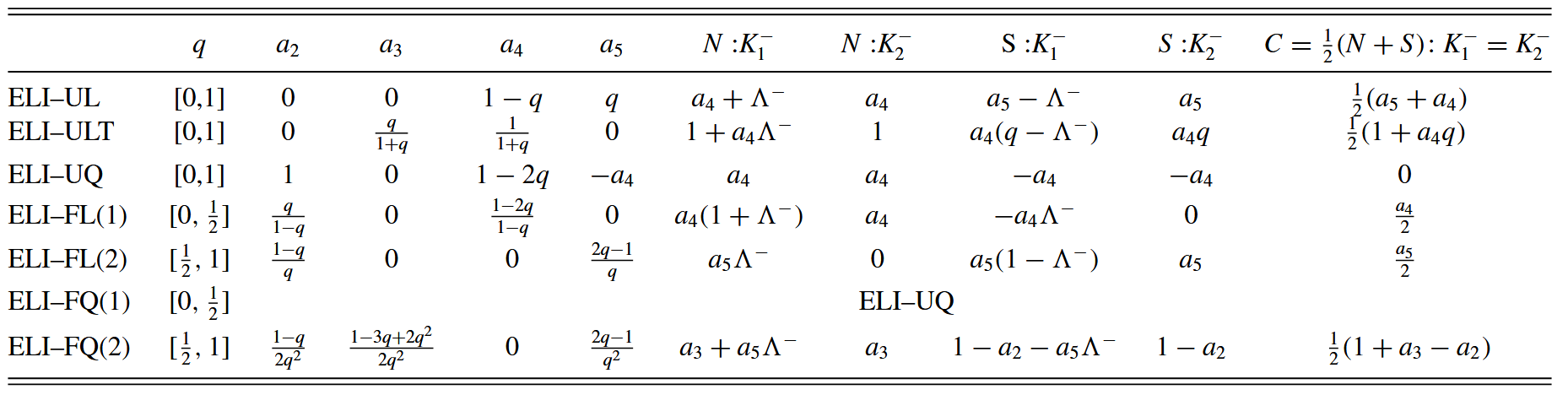
The following table shows the interpolation coefficients provided by Marson et al. [1]. It should be noted that K − K^{-} K − τ + → 1 2 \tau^{+} \rightarrow \frac{1}{2} τ + → 2 1 K − f i ( n e q ) − ( x ⃗ F ) τ − K^{-} \frac{f_{i}^{(neq)-}(\vec{x}_F)}{\tau^{-}} K − τ − f i ( n e q ) − ( x F )
[NOTE] : The calculation of K − K^{-} K −
[1] Marson, F., Thorimbert, Y., Chopard, B., Ginzburg, I. & Latt, J. Enhanced single-node lattice Boltzmann boundary condition for fluid flows . Phys. Rev. E 103, 053308 (2021).格子Boltzmann方法的原理及应用 . (科学出版社, 2009).Boundary conditions for kinetic theory based models I: Lattice boltzmann models . Multiscale Modeling & Simulation 17, 854–872 (2019).One-point second-order curved boundary condition for lattice Boltzmann simulation of suspended particles . Computers & Mathematics with Applications 76, 1593–1607 (2018).